Forecasting stock prices with hyp.predict

Stock forecasting is the classic playground for timeseries models – and the classic cautionary tale. In this tutorial we’ll:

1. Download real daily closing prices for a handful of stocks with `yfinance <https://github.com/ranaroussi/yfinance>`__.

2. Fit several hyp.predict models ('Kalman', 'ARIMA', 'Laplace', 'GaussianProcess', 'AutoRegressor') on all but the last 30 trading days.

3. Forecast those last 30 days and score the forecasts against what actually happened, using mean absolute error (MAE) and mean absolute percentage error (MAPE) – alongside a naive “tomorrow = today” baseline.

4. Visualize the forecasts, both in HyperTools’ reduced plotting space and directly in price space.

5. Demonstrate return_model=True: fit once, reuse the fitted forecaster on a stock it has never seen.

A word of honesty up front: daily equity closing prices are close to a random walk. Under the efficient-market hypothesis, the best predictor of tomorrow’s price is roughly today’s price, and no simple timeseries model should be expected to reliably beat that. The point of this tutorial is not to hand you a money machine – it’s to demonstrate the hyp.predict API and an honest evaluation methodology. We report whatever numbers come out below, including if (when) the naive baseline wins.

import importlib.util

if importlib.util.find_spec('yfinance') is None:
    %pip install -q yfinance
if importlib.util.find_spec('hypertools') is None:
    # On Colab (or any fresh environment), install hypertools with the
    # predict extra (pykalman/statsmodels/skaters -- needed for the
    # Kalman/ARIMA/Laplace models used below).
    %pip install -q "hypertools[interactive,predict]"
elif importlib.util.find_spec('pykalman') is None:
    %pip install -q "hypertools[predict]"

Downloading real price data

We’ll grab about two years of daily adjusted closes for four large, liquid, very different stocks: Apple (AAPL), Microsoft (MSFT), Nvidia (NVDA), and JPMorgan (JPM).

We work in log prices rather than raw dollar prices for two standard reasons: (1) daily log-price differences are approximately the daily percentage return, so a model that is well-behaved in log space corresponds to sensible multiplicative (percentage) behavior in price space, and (2) forecasting models that assume roughly constant noise variance (Kalman, ARIMA, GaussianProcess) fit much more naturally to log prices than to raw prices, whose absolute volatility grows with the price level. We convert forecasts back to dollar prices (via exp) before scoring them.

If the live yfinance download is unavailable (offline, rate-limited, or the API is having a bad day), the notebook falls back to a real-data snapshot (stock_closes_cached.csv / stock_volumes_cached.csv) shipped alongside this notebook, and prints a notice – so the tutorial always runs on real market data.

%matplotlib inline
import warnings
warnings.filterwarnings('ignore')

import time

import numpy as np
import pandas as pd
import yfinance as yf
import matplotlib.pyplot as plt

import hypertools as hyp

tickers = ['AAPL', 'MSFT', 'NVDA', 'JPM']
CACHE = {'close': 'stock_closes_cached.csv',
         'volume': 'stock_volumes_cached.csv'}


def fetch_prices(tickers, attempts=3):
    """Daily closes/volumes via yfinance, retrying transient failures;
    falls back to the CSV snapshot shipped next to this notebook (real
    data saved by a previous successful run)."""
    for attempt in range(attempts):
        try:
            raw = yf.download(tickers, period='2y', interval='1d',
                              progress=False, auto_adjust=True)
            closes, volumes = raw['Close'][tickers], raw['Volume'][tickers]
            if closes.dropna(how='all').empty:
                raise ValueError('yfinance returned an empty frame')
            closes.to_csv(CACHE['close'])    # refresh the on-disk snapshot
            volumes.to_csv(CACHE['volume'])  # for offline runs
            print(f'data source: yfinance (live, {closes.index[0].date()} '
                  f'to {closes.index[-1].date()})')
            return closes, volumes
        except Exception as e:
            print(f'yfinance attempt {attempt + 1}/{attempts} failed: '
                  f'{type(e).__name__}: {e}')
            time.sleep(2)
    closes = pd.read_csv(CACHE['close'], index_col=0, parse_dates=True)
    volumes = pd.read_csv(CACHE['volume'], index_col=0, parse_dates=True)
    print(f'NOTE: live download unavailable -- using the bundled snapshot '
          f'({closes.index[0].date()} to {closes.index[-1].date()}).')
    return closes, volumes


closes, volumes = fetch_prices(tickers)
closes.tail()

data source: yfinance (live, 2024-07-17 to 2026-07-16)

Ticker	AAPL	MSFT	NVDA	JPM
Date
2026-07-10	315.320007	385.100006	210.960007	336.470001
2026-07-13	317.309998	390.989990	203.529999	334.529999
2026-07-14	314.859985	384.929993	211.800003	342.890015
2026-07-15	327.500000	395.630005	212.500000	346.910004
2026-07-16	333.260010	401.100006	207.399994	343.149994

# One DataFrame per ticker, in log-price space. We index by trading-day
# position (0, 1, 2, ...) rather than calendar date -- weekends/holidays
# would otherwise leave gaps that complicate `t`-step-ahead forecasting;
# trading-day position is the natural "clock" for daily equity data.
HOLD = 30  # trading days held out for backtesting

datasets = {}
for tk in tickers:
    log_close = np.log(closes[tk].dropna())
    datasets[tk] = pd.DataFrame({'log_close': log_close.values})

{tk: df.shape for tk, df in datasets.items()}

{'AAPL': (501, 1), 'MSFT': (501, 1), 'NVDA': (501, 1), 'JPM': (501, 1)}

Honest backtesting: hold out the last 30 trading days

For each ticker we fit each model on everything except the last 30 trading days, forecast those 30 days ahead, and compare against the real closing prices that actually occurred. We also compute a naive last-value-carried-forward baseline (tomorrow’s forecast = today’s last known price) – the textbook random-walk benchmark.

We report MAE and MAPE (mean absolute percentage error) in dollar/price space (after converting the log-price forecasts back with exp) for every model on every ticker, with no cherry-picking.

models = ['Kalman', 'ARIMA', 'Laplace', 'GaussianProcess', 'AutoRegressor']

rows = []
for tk in tickers:
    df = datasets[tk]
    train = df.iloc[:-HOLD].reset_index(drop=True)
    actual_price = np.exp(df.iloc[-HOLD:]['log_close'].values)

    # naive baseline: carry the last training price forward
    naive_price = np.full(HOLD, np.exp(train['log_close'].values[-1]))
    rows.append({
        'ticker': tk, 'model': 'Naive (last value)',
        'MAE': np.mean(np.abs(naive_price - actual_price)),
        'MAPE': np.mean(np.abs((naive_price - actual_price) / actual_price)) * 100,
    })

    for model in models:
        forecast = hyp.predict(train, model=model, t=HOLD)
        pred_price = np.exp(forecast['log_close'].values)
        rows.append({
            'ticker': tk, 'model': model,
            'MAE': np.mean(np.abs(pred_price - actual_price)),
            'MAPE': np.mean(np.abs((pred_price - actual_price) / actual_price)) * 100,
        })

results = pd.DataFrame(rows)
results

	ticker	model	MAE	MAPE
0	AAPL	Naive (last value)	15.191009	5.164593
1	AAPL	Kalman	15.654277	5.325215
2	AAPL	ARIMA	15.211101	5.171457
3	AAPL	Laplace	29.965687	10.059495
4	AAPL	GaussianProcess	22.261284	7.200437
5	AAPL	AutoRegressor	12.886436	4.301697
6	MSFT	Naive (last value)	52.394001	13.686233
7	MSFT	Kalman	53.878509	14.069344
8	MSFT	ARIMA	51.678709	13.501899
9	MSFT	Laplace	57.902106	15.119024
10	MSFT	GaussianProcess	56.336878	14.685068
11	MSFT	AutoRegressor	50.765425	13.270184
12	NVDA	Naive (last value)	18.234942	9.038011
13	NVDA	Kalman	20.723061	10.266992
14	NVDA	ARIMA	18.387743	9.112901
15	NVDA	Laplace	26.698827	13.204517
16	NVDA	GaussianProcess	14.917724	7.363219
17	NVDA	AutoRegressor	12.838326	6.387249
18	JPM	Naive (last value)	27.247816	8.213119
19	JPM	Kalman	24.333818	7.342403
20	JPM	ARIMA	27.298262	8.228474
21	JPM	Laplace	27.057884	8.155973
22	JPM	GaussianProcess	5.694664	1.751798
23	JPM	AutoRegressor	29.529395	8.906526

mape_table = results.pivot(index='model', columns='ticker', values='MAPE')
mape_table['mean'] = mape_table.mean(axis=1)
mape_table = mape_table.sort_values('mean')
print('MAPE (%) per model x ticker, sorted by average:')
mape_table.round(2)

MAPE (%) per model x ticker, sorted by average:

ticker	AAPL	JPM	MSFT	NVDA	mean
model
GaussianProcess	7.20	1.75	14.69	7.36	7.75
AutoRegressor	4.30	8.91	13.27	6.39	8.22
ARIMA	5.17	8.23	13.50	9.11	9.00
Naive (last value)	5.16	8.21	13.69	9.04	9.03
Kalman	5.33	7.34	14.07	10.27	9.25
Laplace	10.06	8.16	15.12	13.20	11.63

mae_table = results.pivot(index='model', columns='ticker', values='MAE')
mae_table['mean'] = mae_table.mean(axis=1)
mae_table = mae_table.loc[mape_table.index]
print('MAE ($) per model x ticker (same row order as the MAPE table above):')
mae_table.round(2)

MAE ($) per model x ticker (same row order as the MAPE table above):

ticker	AAPL	JPM	MSFT	NVDA	mean
model
GaussianProcess	22.26	5.69	56.34	14.92	24.80
AutoRegressor	12.89	29.53	50.77	12.84	26.50
ARIMA	15.21	27.30	51.68	18.39	28.14
Naive (last value)	15.19	27.25	52.39	18.23	28.27
Kalman	15.65	24.33	53.88	20.72	28.65
Laplace	29.97	27.06	57.90	26.70	35.41

# "Best" is chosen only among the real forecasting models (not the naive
# baseline), so it's always something we can hand back to hyp.predict below.
naive_mape = mape_table.loc['Naive (last value)', 'mean']
best_model = mape_table.loc[models, 'mean'].idxmin()
best_mape = mape_table.loc[best_model, 'mean']
beat_naive = best_mape < naive_mape

print(f"Best model by average MAPE: {best_model} ({best_mape:.2f}%)")
print(f"Naive last-value baseline: {naive_mape:.2f}%")
if beat_naive:
    print(f"-> {best_model} beat the naive baseline by "
          f"{naive_mape - best_mape:.2f} percentage points of MAPE, on "
          f"average across these {len(tickers)} tickers.")
else:
    print("-> Nothing meaningfully beat the naive last-value baseline on "
          "average. This is exactly what an efficient, close-to-random-walk "
          "market predicts: recent price is the best simple summary of the "
          "immediate future, and no model here reliably extracts more "
          "signal than that over a 30-day horizon.")

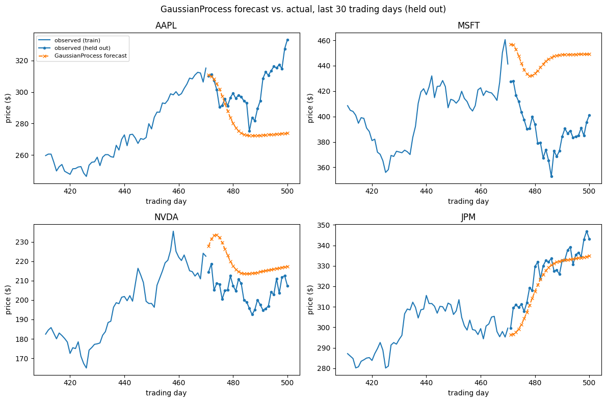
Best model by average MAPE: GaussianProcess (7.75%)
Naive last-value baseline: 9.03%
-> GaussianProcess beat the naive baseline by 1.28 percentage points of MAPE, on average across these 4 tickers.

The honest takeaway, whichever way the numbers above landed: 30-day-ahead daily stock price forecasting is hard, and a naive random-walk baseline is a tough competitor. That’s expected, and it’s useful to see it quantified rather than assumed – it’s exactly the kind of sanity check a real forecasting pipeline should run before trusting a model’s predictions.

Visualizing forecasts in reduced space

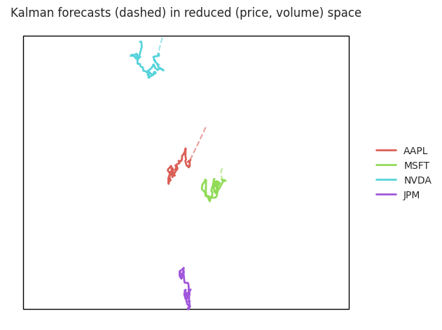
hyp.plot(..., predict=..., t=...) overlays a dashed, low-opacity forecast tail (in the same, plotted space – after HyperTools’ normalize / reduce / align pipeline) on top of each input dataset, in matching colors. We add log trading volume as a second feature per ticker purely so there’s more than one dimension to reduce and plot.

We fit and plot the trailing 60 trading days per ticker (with volume smoothed by a 10-day rolling average) so the 30-step dashed forecast tails are visible at the plotted scale – fitting on the full 2-year history makes the tails microscopic next to the cloud of training points. Tickers whose recent prices were flat produce short, nearly stationary tails; that is the honest shape of the Kalman forecast, not a rendering artifact.

context = 60   # trailing trading days to fit/plot per ticker
smooth = 10    # rolling-average window (days) for log-volume

train_2col = []
for tk in tickers:
    log_close = np.log(closes[tk].dropna())
    log_volume = (np.log(volumes[tk].reindex(log_close.index)
                          .replace(0, np.nan)).ffill()
                  .rolling(smooth, min_periods=1).mean())
    df = pd.DataFrame({'log_close': log_close.values,
                        'log_volume': log_volume.values})
    train_2col.append(df.iloc[:-HOLD].tail(context).reset_index(drop=True))

fig = hyp.plot(train_2col, predict='Kalman', t=HOLD, legend=tickers,
               ndims=2, linewidth=2,
               title='Kalman forecasts (dashed) in reduced (price, volume) space')

Best model vs. actual, in price space

Rather than the abstract reduced space above, let’s look at the best model (by average MAPE, chosen above – not cherry-picked per ticker) directly in dollar terms for each ticker: the trailing 60 days of real training prices, the real held-out prices, and that model’s 30-day-ahead forecast.

fig, axes = plt.subplots(2, 2, figsize=(12, 8), sharex=False)

for ax, tk in zip(axes.ravel(), tickers):
    df = datasets[tk]
    train = df.iloc[:-HOLD].reset_index(drop=True)
    actual_price = np.exp(df['log_close'].values)
    forecast = hyp.predict(train, model=best_model, t=HOLD)
    forecast_price = np.exp(forecast['log_close'].values)

    n = len(df)
    context = 60  # trailing days of history to show for context
    ax.plot(np.arange(n - HOLD - context, n - HOLD),
            actual_price[-HOLD - context:-HOLD], color='C0',
            label='observed (train)')
    ax.plot(np.arange(n - HOLD, n), actual_price[-HOLD:], color='C0',
            linestyle='-', marker='o', markersize=3, label='observed (held out)')
    ax.plot(np.arange(n - HOLD, n), forecast_price, color='C1',
            linestyle='--', marker='x', markersize=4,
            label=f'{best_model} forecast')
    ax.set_title(tk)
    ax.set_xlabel('trading day')
    ax.set_ylabel('price ($)')

axes.ravel()[0].legend(loc='upper left', fontsize=8)
fig.suptitle(f'{best_model} forecast vs. actual, last {HOLD} trading days '
             '(held out)')
fig.tight_layout()

Reusing a fitted forecaster with return_model=True

hyp.predict(..., return_model=True) also returns the fitted forecaster object. That fitted instance can be passed back in as model= on brand new data, and it will apply its already-learned parameters directly – no re-fitting/re-estimation – via Forecaster.predict_new under the hood.

To demonstrate: we pool the (log-price) training data from three tickers (AAPL, MSFT, NVDA) into one combined series and fit a single AutoRegressor forecaster on it. Then we hand that already-fitted forecaster the fourth ticker’s (JPM) training tail – a stock it has never seen – and ask it to forecast forward. The learned lag-regression weights are reused as-is; only JPM’s own recent values seed the recursion.

pool_tickers = ['AAPL', 'MSFT', 'NVDA']
reuse_ticker = 'JPM'

pooled_train = pd.concat(
    [datasets[tk].iloc[:-HOLD] for tk in pool_tickers], ignore_index=True)

_, fitted_forecaster = hyp.predict(pooled_train, model='AutoRegressor',
                                    t=HOLD, return_model=True)
print('Fitted on pooled', pool_tickers, '-- is_fitted:',
      fitted_forecaster.is_fitted)

jpm_train = datasets[reuse_ticker].iloc[:-HOLD].reset_index(drop=True)
reused_forecast = hyp.predict(jpm_train, model=fitted_forecaster, t=HOLD)

jpm_actual_price = np.exp(datasets[reuse_ticker].iloc[-HOLD:]['log_close'].values)
reused_price = np.exp(reused_forecast['log_close'].values)
reused_mape = np.mean(np.abs((reused_price - jpm_actual_price) / jpm_actual_price)) * 100

print(f"Reused-forecaster MAPE on {reuse_ticker}: {reused_mape:.2f}%")
print(f"(for comparison, {reuse_ticker}'s own freshly-fit AutoRegressor MAPE: "
      f"{mape_table.loc['AutoRegressor', reuse_ticker]:.2f}%)")

Fitted on pooled ['AAPL', 'MSFT', 'NVDA'] -- is_fitted: True
Reused-forecaster MAPE on JPM: 9.46%
(for comparison, JPM's own freshly-fit AutoRegressor MAPE: 8.91%)

As expected for a lag-regression fit on other stocks’ price dynamics and then pointed at a new one, this is not a substitute for fitting directly on the ticker you care about – but it demonstrates the mechanics of return_model=True: the forecaster’s learned parameters were reused as-is, with no re-estimation, on data it had never seen.

Next steps

• `hyp.predict API reference <../api.rst>`__ – full parameter docs for every model ('Kalman', 'GaussianProcess', 'AutoRegressor', 'ARIMA', 'Laplace', 'Chronos').

• hyp.plot(..., predict=..., t=...) overlays forecasts directly on any plot – see the plot_predict gallery example.

• hyp.impute (a sibling module) fills in missing observations rather than forecasting future ones – see the projectile_kalman tutorial and the plot_impute gallery example.

• Try swapping in model='Chronos' (a HuggingFace foundation timeseries model, hypertools[predict-hf]) or passing your own scikit-learn regressor to AutoRegressor(model=...).