# Install hypertools (run this first on Colab)
%pip install -q "hypertools[interactive]"

Clustering with Hypertools

The cluster feature performs clustering analysis on the data (an array, dataframe, or list) and returns a list of cluster labels.

The default clustering model is K-Means (argument ‘KMeans’). Also supported: AffinityPropagation, AgglomerativeClustering, BayesianGaussianMixture, Birch, DBSCAN, FeatureAgglomeration, GaussianMixture, HDBSCAN, LatentDirichletAllocation, MeanShift, MiniBatchKMeans, NMF, OPTICS, and SpectralClustering. (Note that FeatureAgglomeration clusters the features – columns – rather than the observations.)

Note that, if a list is passed, the arrays will be stacked and clustering will be performed across all lists (not within each list).

Import Packages

import hypertools as hyp
from collections import Counter

%matplotlib inline

Load your data

We will load one of the sample datasets. This dataset consists of 8,124 samples of mushrooms with various text features.

mushrooms = hyp.load('mushrooms')

We can peek at the first few rows of the dataframe using the pandas function head()

mushrooms.head()

	bruises	cap-color	cap-shape	cap-surface	gill-attachment	gill-color	gill-size	gill-spacing	habitat	odor	...	ring-type	spore-print-color	stalk-color-above-ring	stalk-color-below-ring	stalk-root	stalk-shape	stalk-surface-above-ring	stalk-surface-below-ring	veil-color	veil-type
0	t	n	x	s	f	k	n	c	u	p	...	p	k	w	w	e	e	s	s	w	p
1	t	y	x	s	f	k	b	c	g	a	...	p	n	w	w	c	e	s	s	w	p
2	t	w	b	s	f	n	b	c	m	l	...	p	n	w	w	c	e	s	s	w	p
3	t	w	x	y	f	n	n	c	u	p	...	p	k	w	w	e	e	s	s	w	p
4	f	g	x	s	f	k	b	w	g	n	...	e	n	w	w	e	t	s	s	w	p

5 rows × 22 columns

Obtain cluster labels

To obtain cluster labels, simply pass the data to hyp.cluster. Since we have not specified a desired number of clusters, the default of 3 clusters is used (labels 0, 1, and 2). Additionally, since we have not specified a desired clustering algorithm, K-Means is used by default.

labels = hyp.cluster(mushrooms)
set(labels)

{np.int32(0), np.int32(1), np.int32(2)}

We can further examine the number of datapoints assigned each label.

Counter(labels)

Counter({np.int32(2): 3269, np.int32(1): 3105, np.int32(0): 1750})

Specify number of cluster labels

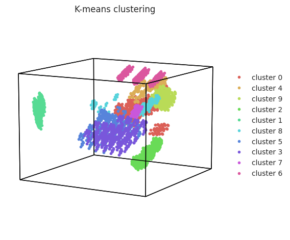
You can also specify the number of desired clusters by setting the n_clusters argument to an integer number of clusters, as below. We can see that when we pass the int 10 to n_clusters, 10 cluster labels are assigned.

Since we have not specified a desired clustering algorithm, K-Means is used by default.

labels_10 = hyp.cluster(mushrooms, n_clusters = 10)
set(labels_10)

{np.int32(0),
 np.int32(1),
 np.int32(2),
 np.int32(3),
 np.int32(4),
 np.int32(5),
 np.int32(6),
 np.int32(7),
 np.int32(8),
 np.int32(9)}

Different clustering models

You may prefer to use a clustering model other than K-Means. To do so, simply pass a string to the cluster argument specifying the desired clustering algorithm.

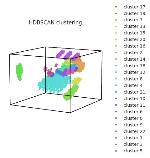
In this case, we specify the clustering model (HDBSCAN). Note that HDBSCAN determines the number of clusters directly from the data, so we don’t pass n_clusters (it would be ignored).

labels_HDBSCAN = hyp.cluster(mushrooms, cluster='HDBSCAN')

fig = hyp.plot(mushrooms, '.', hue=[f'cluster {label}' for label in labels_10],
               legend=True, title='K-means clustering')
fig2 = hyp.plot(mushrooms, '.', hue=[f'cluster {label}' for label in labels_HDBSCAN],
               legend=True, title='HDBSCAN clustering')