# Install hypertools (run this first on Colab)
import importlib.util
if importlib.util.find_spec('hypertools') is None:
    %pip install -q "hypertools[interactive]"

Modern scikit-learn models and dynamical systems

HyperTools 1.0 exposes the latest scikit-learn models directly through its plotting interface. In this tutorial we’ll use sklearn’s built-in HDBSCAN for density-based clustering, Gaussian mixture models for soft clustering, and then visualize the dynamics of the Lorenz attractor using time-delay embeddings. No extra dependencies are needed beyond HyperTools itself.

%matplotlib inline
import warnings
warnings.filterwarnings('ignore')

import numpy as np
from scipy.integrate import solve_ivp
from sklearn.datasets import make_blobs, make_moons

import hypertools as hyp

Density-based clustering with HDBSCAN

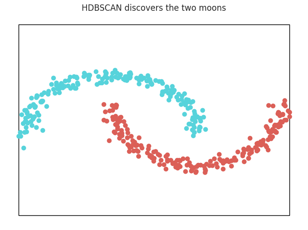
HDBSCAN finds clusters of varying density without needing to know the number of clusters in advance – and as of scikit-learn 1.3 it’s built right in. K-means famously fails on the “two moons” dataset; HDBSCAN handles it gracefully. Just pass cluster='HDBSCAN' (no n_clusters needed):

moons, _ = make_moons(n_samples=400, noise=0.06, random_state=42)
fig = hyp.plot(moons, 'o', ndims=2, cluster='HDBSCAN',
               title='HDBSCAN discovers the two moons')

Soft clustering with Gaussian mixture models

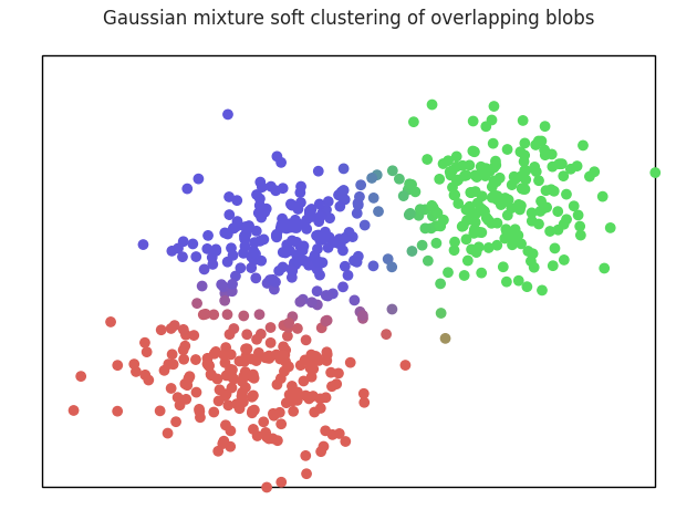
Hard clustering assigns every point to exactly one cluster. But real data is often ambiguous! When you pass cluster='GaussianMixture', HyperTools colors each observation by its proportional blend of cluster memberships. On overlapping blobs, points between clusters take on intermediate colors:

blobs, _ = make_blobs(n_samples=600, centers=3, cluster_std=2.5,
                      random_state=17)
fig = hyp.plot(blobs, 'o', ndims=2, cluster='GaussianMixture', n_clusters=3,
               title='Gaussian mixture soft clustering of overlapping blobs')

Visualizing dynamics: the Lorenz attractor

HyperTools is also great for visualizing how systems evolve over time. Here we’ll integrate the classic Lorenz system with scipy:

def lorenz(t, state, sigma=10.0, rho=28.0, beta=8.0 / 3.0):
    x, y, z = state
    return [sigma * (y - x), x * (rho - z) - y, x * y - beta * z]

t = np.linspace(0, 50, 5000)
sol = solve_ivp(lorenz, (t[0], t[-1]), [1.0, 1.0, 1.0], t_eval=t)
trajectory = sol.y.T  # 5000 timepoints x 3 dimensions
trajectory.shape

(5000, 3)

Suppose we could only observe a single coordinate of the system. Takens’ embedding theorem says we can still recover the attractor’s geometry by building a time-delay embedding: stacking time-lagged copies of the observed coordinate into a matrix. HyperTools takes care of projecting that high-dimensional delay matrix back down to 3D.

Passing a continuous array as hue draws the trajectory as a multicolored line, so color traces the passage of time:

x = trajectory[:, 0]  # observe only the x-coordinate
tau, dims = 5, 20     # delay length and embedding dimension
n = len(x) - tau * (dims - 1)
delay_matrix = np.column_stack([x[i * tau:i * tau + n] for i in range(dims)])

fig = hyp.plot(delay_matrix, hue=np.arange(n, dtype=float),
               title='Lorenz attractor from a time-delay embedding')

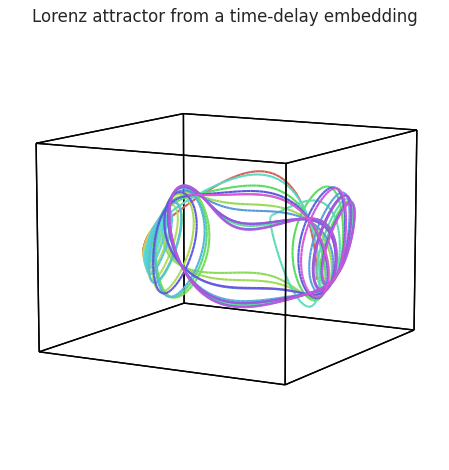
The butterfly-shaped attractor emerges from just one observed coordinate!

Animating a trajectory

Finally, let’s animate the trajectory itself. With animate=True, HyperTools sweeps a moving window along the timeseries – slowly, over 30 seconds at 30 frames per second. We export the animation as an MP4 (compact and fast to render), then convert it to a GIF with ffmpeg for inline display:

fig, ani = hyp.plot(trajectory, animate=True, duration=30, frame_rate=30,
               save_path='lorenz_trajectory.mp4', show=False)

import os
import shutil
import subprocess

if shutil.which('ffmpeg'):
    filters = ('fps=30,scale=420:-1:flags=lanczos,split [a][b]; '
               '[a] palettegen=max_colors=64 [p]; '
               '[b][p] paletteuse=dither=bayer:bayer_scale=3')
    subprocess.run(['ffmpeg', '-y', '-i', 'lorenz_trajectory.mp4',
                    '-vf', filters, 'lorenz_trajectory.gif'],
                   check=True, capture_output=True)
    os.remove('lorenz_trajectory.mp4')
    print(f"gif: {os.path.getsize('lorenz_trajectory.gif')/1e6:0.1f} MB")
else:
    print('ffmpeg not found -- skipping GIF conversion; the animation '
          'is saved as lorenz_trajectory.mp4 instead.')

gif: 9.0 MB

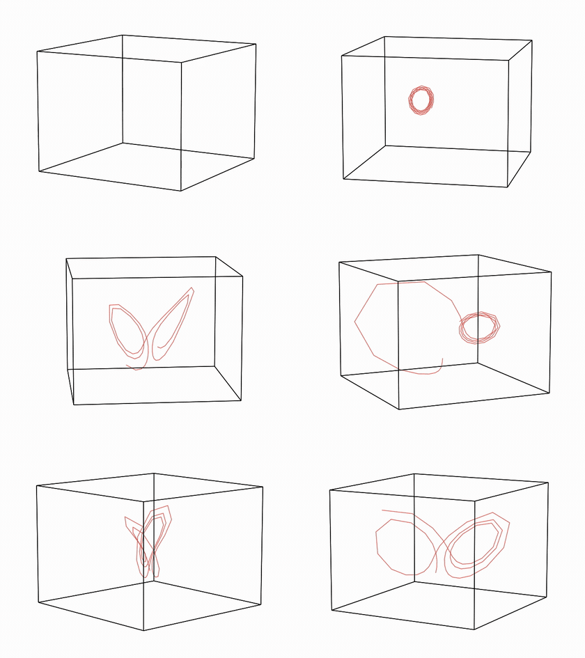
(The animation above is loaded from ``lorenz_trajectory.gif``, written by the cell above; if your environment does not render it inline, open the file directly.)

Next steps

Try animate='spin' for a rotating view, chemtrails=True to add a fading tail to animated trajectories, or cluster the delay matrix itself with cluster='HDBSCAN' to segment the attractor’s lobes.