# Install hypertools (run this first on Colab)
%pip install -q "hypertools[interactive]"

[notice] A new release of pip is available: 25.3 -> 26.1.2
[notice] To update, run: /Users/jmanning/hypertools/.venv/bin/python -m pip install --upgrade pip
Note: you may need to restart the kernel to use updated packages.

Plotting streaming data

HyperTools treats data streams as just another supported data type: pass any Python iterator/generator, or a Hugging Face streaming dataset (load_dataset(..., streaming=True)), directly to hyp.plot – no special flag needed.

How it works (see issue #101):

1. the first stream_init samples (default 10,000) are used to estimate the normalization and dimensionality-reduction parameters;

2. those fitted models are then applied to every subsequent sample, which is added to the plot dynamically as it arrives;

3. streaming continues until the stream is exhausted, stream_max samples have been consumed, or you interrupt with Ctrl-C. Infinite streams render continually – and if you’re saving an animation with save_path, the file is finalized whenever streaming stops (including on interrupt).

Because new samples are projected with models fitted on the head of the stream, the reduction model must support transform() (e.g. the default IncrementalPCA, or PCA/UMAP – but not TSNE).

import numpy as np
import hypertools as hyp

%matplotlib inline

Streaming from a generator

Here’s a simulated live data feed: a Lorenz attractor unfolding in a 10-dimensional embedding, written as an infinite generator. hyp.plot detects that it’s a stream, fits IncrementalPCA on the first 500 samples, then projects each new chunk of 100 samples through that fitted model and adds it to the plot. stream_max cuts the (infinite) stream off so the animation can be saved.

def live_feed(dt=0.01, dim=10, seed=42):
    """An infinite stream: Lorenz dynamics embedded in `dim` dimensions."""
    rng = np.random.default_rng(seed)
    W = rng.standard_normal((3, dim))
    xyz = np.array([1., 1., 1.])
    while True:
        x, y, z = xyz
        xyz = xyz + dt * np.array([10 * (y - x),
                                   x * (28 - z) - y,
                                   x * y - 8 / 3 * z])
        yield xyz @ W + 0.05 * rng.standard_normal(dim)


fig = hyp.plot(live_feed(), stream_init=500, stream_chunk=100,
               stream_max=3000, save_path='streaming_lorenz.gif',
               show=False)
fig.stream_info['n_samples'], fig.stream_info['xform_data'][0].shape

(3000, (3000, 3))

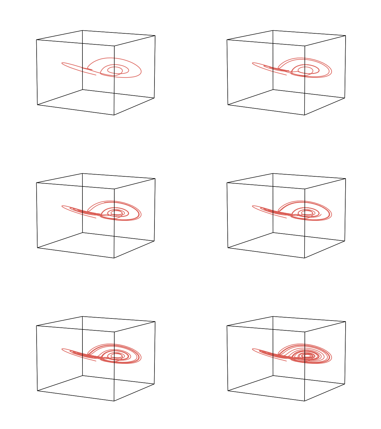
Each animation frame corresponds to one fetched chunk, so stream_chunk sets both the download batch size and the temporal resolution of the saved animation.

The returned figure retains everything that was consumed via fig.stream_info: fig.stream_info['data'] holds the raw samples, fig.stream_info['xform_data'] the projected trajectory, and fig.stream_info['n_samples'] / ['reduce_model'] / ['truncated'] record the number of samples seen, the fitted reduction model, and whether the stream was cut off (truncated=True means there was more data left).

{k: (type(v).__name__ if k == 'reduce_model' else
     (v[0].shape if k in ('data', 'xform_data') else v))
 for k, v in fig.stream_info.items()}

{'data': (3000, 10),
 'xform_data': (3000, 3),
 'n_samples': 3000,
 'reduce_model': 'IncrementalPCA',
 'truncated': True}

Comet-style display with stream_window

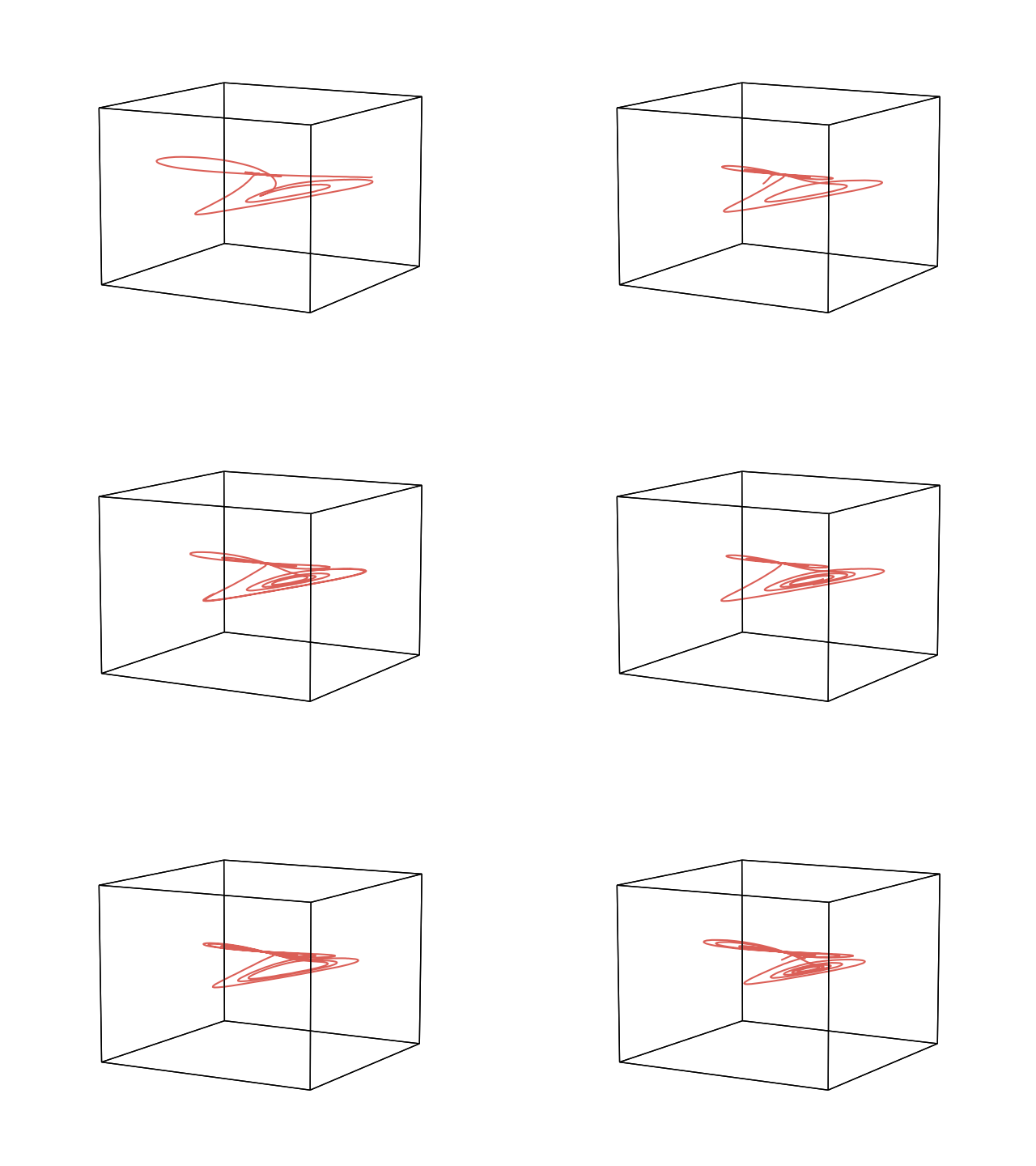
For long (or infinite) streams the accumulated trajectory can get dense. Passing stream_window displays only the most recent samples – older points scroll off comet-style – while everything consumed is still retained on the returned figure’s stream_info.

fig = hyp.plot(live_feed(seed=7), stream_init=500, stream_chunk=100,
               stream_max=3000, stream_window=750,
               save_path='streaming_window.gif', show=False)
len(fig.axes[0].lines[0].get_data_3d()[0]), fig.stream_info['xform_data'][0].shape[0]

(750, 3000)

Streaming a Hugging Face dataset

Any datasets.IterableDataset streams straight into hyp.plot without downloading the full dataset first. Rows arrive as dicts; numeric fields are extracted (in order) and concatenated into one vector per sample, and non-numeric fields are ignored – use .select_columns(...) to control exactly which features are used.

from datasets import load_dataset

ds = load_dataset('scikit-learn/iris', split='train', streaming=True)
ds = ds.select_columns(['SepalLengthCm', 'SepalWidthCm',
                        'PetalLengthCm', 'PetalWidthCm'])

fig = hyp.plot(ds, '.', markersize=6, stream_init=50, stream_chunk=25)
fig.stream_info['n_samples'], fig.stream_info['data'][0].shape

Warning: You are sending unauthenticated requests to the HF Hub. Please set a HF_TOKEN to enable higher rate limits and faster downloads.

(150, (150, 4))

The four numeric iris measurements stream through the model fitted on the first 50 flowers and land in a 3-dimensional embedding, 50 → 150 samples, without the dataset ever being materialized locally.

A few practical notes:

• with the default stream_max=None, plotting an infinite stream runs until you interrupt it (Ctrl-C) – the plot keeps updating live, and any save_path animation is finalized on interrupt;

• when stream_max is set, hypertools peeks one sample past the limit to determine whether the stream was truncated, so budget for one extra sample being consumed from costly or stateful sources;

• align and cluster aren’t yet supported for streams (a stream is a single dataset, and clustering streams is planned for a future release);

• everything consumed is kept in memory on the returned figure’s stream_info, so very long-running streams should budget accordingly.