# Install hypertools (run this first on Colab)
import importlib.util
if importlib.util.find_spec('hypertools') is None:
    %pip install -q "hypertools[interactive]"

# This tutorial also uses sentence-transformers (not a HyperTools dep);
# self-install it so a top-to-bottom run works headlessly too.
if importlib.util.find_spec('sentence_transformers') is None:
    %pip install -q sentence-transformers

Mapping Wikipedia with modern text embeddings

Text embedding models map documents into high-dimensional vector spaces where nearby vectors correspond to semantically related documents. In this tutorial we’ll embed HyperTools’ sample corpus of Wikipedia articles using a modern text embedding model (`BAAI/bge-small-en-v1.5 <https://huggingface.co/BAAI/bge-small-en-v1.5>`__), untangle the embedding space with UMAP, discover article groupings with soft (Gaussian mixture) clustering, and explore the resulting “map” of Wikipedia in 3D.

This tutorial uses one extra library that is not installed with HyperTools. You can install it by running:

%pip install sentence-transformers

(The animation step at the end also uses ffmpeg to convert the exported movie into a GIF.)

%matplotlib inline
import os
os.environ['HF_HUB_DISABLE_PROGRESS_BARS'] = '1'
os.environ['HF_HUB_VERBOSITY'] = 'error'
os.environ['TOKENIZERS_PARALLELISM'] = 'false'

import warnings
warnings.filterwarnings('ignore')

import numpy as np
from sentence_transformers import SentenceTransformer

import hypertools as hyp

Loading the sample Wikipedia corpus

HyperTools ships with a sample corpus of Wikipedia articles, available through hyp.load('wiki'). The loader returns the raw data directly – a list containing one array of documents, where each entry is the (preprocessed) text of one Wikipedia article.

wiki = hyp.load('wiki')
articles = [str(doc) for doc in wiki[0].ravel()]

print(f'number of articles: {len(articles)}')
print(f'average article length: {np.mean([len(a) for a in articles]):0.0f} characters')
print('\nfirst article (excerpt):\n', articles[0][:250], '...')

number of articles: 3136
average article length: 18048 characters

first article (excerpt):
 a gun salute is the most commonly recognized of the customary gun salutes that are performed by the firing of cannons or artillery as a military honorthe custom stems from naval tradition where a warship would fire its cannons harmlessly out to sea u ...

Embedding the articles

We’ll embed each article with `BAAI/bge-small-en-v1.5 <https://huggingface.co/BAAI/bge-small-en-v1.5>`__, a compact but powerful sentence-embedding model that maps each document onto a 384-dimensional vector. The model reads at most 512 tokens per document, so we truncate each article to its first 2,000 characters (typically about 350-450 tokens, comfortably within the limit) – this also speeds up encoding considerably, and the opening of a Wikipedia article is nearly always a summary of the whole article anyway.

truncated = [a[:2000] for a in articles]

model = SentenceTransformer('BAAI/bge-small-en-v1.5')
embeddings = model.encode(truncated, batch_size=64, show_progress_bar=False)
embeddings.shape

(3136, 384)

Mapping the corpus with UMAP and soft clustering

Now we can draw the map – in a single call. Passing reduce='UMAP' projects the 384-dimensional embeddings down to 3D using UMAP, a nonlinear method that is particularly good at untangling text embedding spaces. Passing cluster={'model': 'GaussianMixture', 'n_clusters': 10} fits a 10-component Gaussian mixture model to the embeddings and colors each article by its blend of cluster memberships, automatically: mixture models yield soft assignments, and HyperTools renders each article’s color as an exact per-point blend of the cluster colors, weighted by that article’s mixture proportions. Articles deep inside a cluster take on its pure color, while articles between clusters get smoothly intermediate hues. The '.' format string together with markersize=2 plots each article as a small dot.

UMAP is stochastic: re-fitting it gives a different layout on every call unless it is seeded. We pass random_state=42 (via the dict form of reduce=) so that repeated calls – the static map here and the animated version below – produce the same layout.

fig = hyp.plot(embeddings, '.', markersize=2,
               reduce={'model': 'UMAP', 'kwargs': {'random_state': 42}},
               cluster={'model': 'GaussianMixture', 'n_clusters': 10},
               title='Wikipedia articles (BGE embeddings + UMAP)')

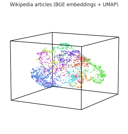
Each dot is one Wikipedia article. Articles about related topics form clumps and filaments, and the blended colors show where topics shade into one another.

Taking a spin around the map

A static projection of a 3D point cloud always hides something. Setting animate='spin' slowly rotates the camera once around the map (over 10 seconds, at 30 frames per second) so we can inspect it from every angle. We export the animation as an MP4 – compact and fast to render – and then convert it to a GIF with ffmpeg for inline display.

fig, ani = hyp.plot(embeddings, '.', markersize=2,
               reduce={'model': 'UMAP', 'kwargs': {'random_state': 42}},
               cluster={'model': 'GaussianMixture', 'n_clusters': 10},
               animate='spin', duration=10, rotations=1, frame_rate=30,
               save_path='wikipedia_embeddings_spin.mp4', show=False)

print(f"mp4: {os.path.getsize('wikipedia_embeddings_spin.mp4')/1e6:0.1f} MB")

mp4: 2.3 MB

import shutil
import subprocess

if shutil.which('ffmpeg'):
    filters = ('fps=30,scale=420:-1:flags=lanczos,split [a][b]; '
               '[a] palettegen=max_colors=64 [p]; '
               '[b][p] paletteuse=dither=bayer:bayer_scale=3')
    subprocess.run(['ffmpeg', '-y', '-i', 'wikipedia_embeddings_spin.mp4',
                    '-vf', filters, 'wikipedia_embeddings_spin.gif'],
                   check=True, capture_output=True)
    os.remove('wikipedia_embeddings_spin.mp4')
    print(f"gif: {os.path.getsize('wikipedia_embeddings_spin.gif')/1e6:0.1f} MB")
else:
    print('ffmpeg not found -- skipping GIF conversion; the animation '
          'is saved as wikipedia_embeddings_spin.mp4 instead.')

gif: 6.5 MB

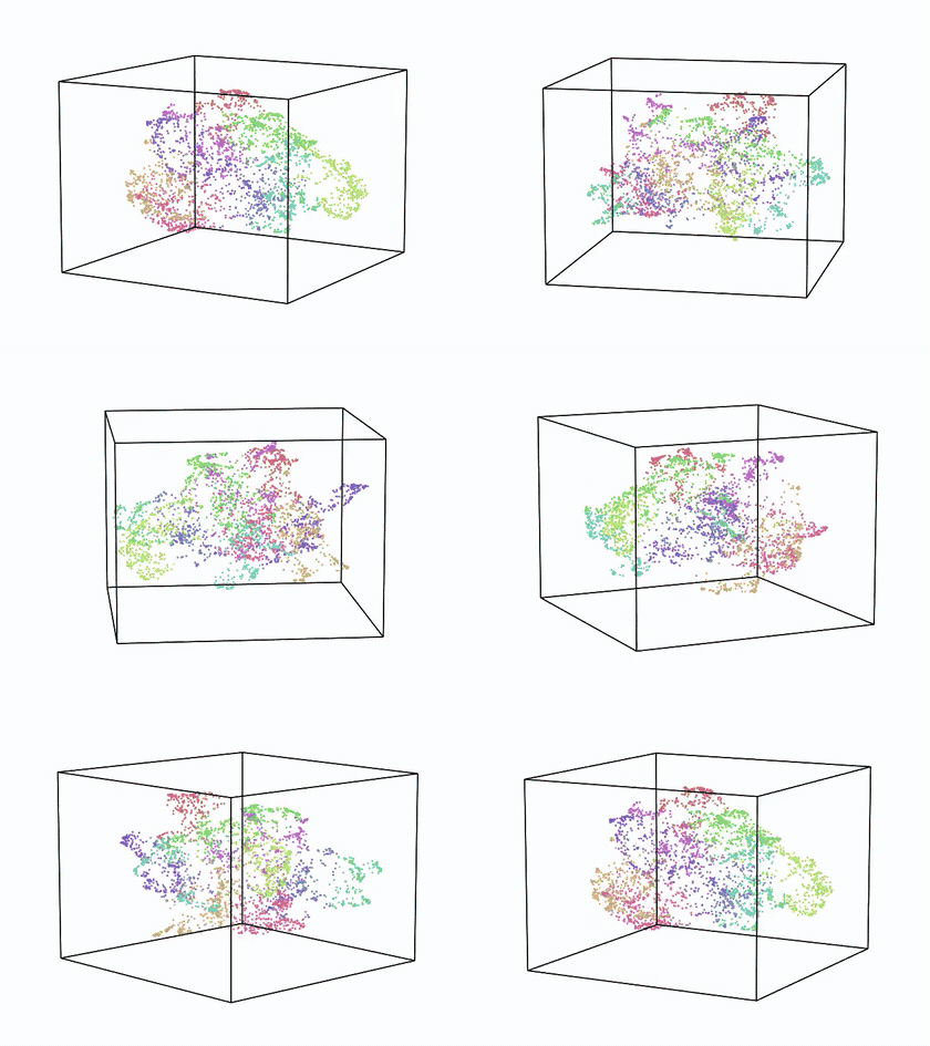
(The animation above is loaded from ``wikipedia_embeddings_spin.gif``, written by the cell above; if your environment does not render it inline, open the file directly.)

Live keywords: mapping fresh articles by category (GH #187)

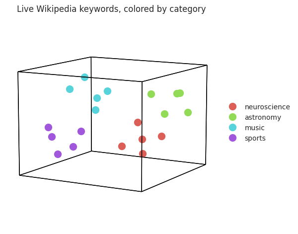
The corpus above is a fixed snapshot bundled with HyperTools. We can also build a corpus on the fly: pick a set of keywords grouped into categories, fetch the current live article for each keyword straight from Wikipedia via the `Wikipedia-API <https://github.com/martin-majlis/Wikipedia-API>`__ package, embed them with the same model as above, and plot the resulting point cloud colored by keyword category – with a volumetric density overlay showing where each category’s articles cluster in embedding space.

import importlib.util
if importlib.util.find_spec('wikipediaapi') is None:
    %pip install -q wikipedia-api

import wikipediaapi

wiki_api = wikipediaapi.Wikipedia(
    user_agent='hypertools-tutorial (https://github.com/ContextLab/hypertools)',
    language='en')

# a keyword set spanning four unrelated categories
keyword_groups = {
    'neuroscience': ['Neuroscience', 'Neuron', 'Cerebral cortex', 'Synapse',
                      'Hippocampus'],
    'astronomy': ['Astronomy', 'Black hole', 'Galaxy', 'Exoplanet', 'Nebula'],
    'music': ['Jazz', 'Classical music', 'Rock music', 'Hip hop music',
              'Opera'],
    'sports': ['Basketball', 'Soccer', 'Tennis', 'Swimming', 'Cricket'],
}

titles, live_texts, categories = [], [], []
for category, keywords in keyword_groups.items():
    for kw in keywords:
        page = wiki_api.page(kw)
        if not page.exists():
            print(f'  (skipping {kw!r}: no such article)')
            continue
        titles.append(kw)
        # the summary is already a clean, self-contained excerpt of the
        # live article -- fall back to the full text for unusually short
        # summaries
        live_texts.append(page.summary if len(page.summary) > 200
                           else page.text)
        categories.append(category)

print(f'fetched {len(titles)} live articles across '
      f'{len(keyword_groups)} categories:')
for title, category in zip(titles, categories):
    print(f'  [{category}] {title}')

fetched 20 live articles across 4 categories:
  [neuroscience] Neuroscience
  [neuroscience] Neuron
  [neuroscience] Cerebral cortex
  [neuroscience] Synapse
  [neuroscience] Hippocampus
  [astronomy] Astronomy
  [astronomy] Black hole
  [astronomy] Galaxy
  [astronomy] Exoplanet
  [astronomy] Nebula
  [music] Jazz
  [music] Classical music
  [music] Rock music
  [music] Hip hop music
  [music] Opera
  [sports] Basketball
  [sports] Soccer
  [sports] Tennis
  [sports] Swimming
  [sports] Cricket

Embedding and mapping the live articles

We reuse the same BAAI/bge-small-en-v1.5 model from above to embed the live articles, then plot them with hue= set to each article’s keyword category – hyp.plot assigns each category a distinct color automatically.

live_truncated = [t[:2000] for t in live_texts]
live_embeddings = model.encode(live_truncated, batch_size=16,
                               show_progress_bar=False)
live_embeddings.shape

(20, 384)

fig = hyp.plot(live_embeddings, '.', markersize=20,
               reduce={'model': 'UMAP', 'kwargs': {'random_state': 42}},
               hue=categories, legend=True,
               title='Live Wikipedia keywords, colored by category')

Volumetric density overlay

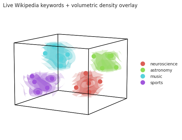
Passing density=True alongside hue= adds a translucent volumetric KDE “glow” around each colored group (GH #108, #191), making it easier to see where each category’s articles concentrate in the embedding space – even with a modest number of live-fetched articles.

Because we seeded UMAP above, this plot has the same layout as the previous one – just with the density overlay added.

fig = hyp.plot(live_embeddings, '.', markersize=20,
               reduce={'model': 'UMAP', 'kwargs': {'random_state': 42}},
               hue=categories, legend=True, density=True,
               title='Live Wikipedia keywords + volumetric density overlay')

Next steps

Try a larger embedding model (e.g. BAAI/bge-base-en-v1.5), a different number of mixture components, or swap UMAP for t-SNE (reduce='TSNE'). You can also explore the map interactively with backend='plotly', or use hyp.plot(..., explore=True) to hover over individual articles.