Imputing and forecasting a real projectile arc with hyp.impute and hyp.predict

A basketball leaving a shooter’s hands and arcing toward the hoop is about as clean a real-world example of projectile motion as you can find: once the ball is in the air, gravity dominates and the trajectory should look like the smooth parabola from an introductory physics class (ignoring the smaller effects of air drag and spin).

In this tutorial we use real optical tracking data – not a simulation – of an actual NBA jump shot:

• Source: linouk23/NBA-Player-Movements, a GitHub re-hosting of the NBA’s SportVU player/ball tracking data from the 2015-16 season. SportVU used an array of optical cameras installed in every NBA arena to record the (x, y, z) position of the ball and all ten players 25 times per second. Cite as: “NBA SportVU player-tracking data (2015-16 season), re-hosted by linouk23/NBA-Player- Movements on GitHub.” We treat this as free for educational/non-commercial use; the repo declares no explicit OSS license, so please check before any commercial reuse.

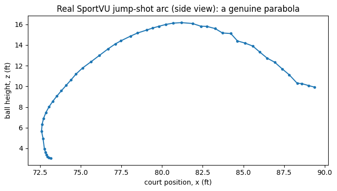
• Extracted arc: game 0021500492 (2016-01-01, Charlotte Hornets @ Toronto Raptors), event index 34, ball moments 226:276 – 50 consecutive frames (2.0 s) of a genuine jump-shot arc. The ball rises from a release height of ~3.1 ft to an apex of ~16.2 ft, then descends toward the far hoop while also moving ~17 ft downcourt and ~19 ft across the court.

Why a Kalman filter for projectile motion?

A constant-acceleration state-space model is a very natural match for ballistic flight: under gravity alone, each coordinate’s acceleration is constant (zero horizontally, -g vertically), so position, velocity, and acceleration together form a simple linear-Gaussian dynamical system – exactly what a Kalman filter models. That makes the Kalman filter a principled choice for two related but distinct tasks on this trajectory:

1. Imputation (hyp.impute(data, model='Kalman')): fill in missing frames – including entire frames where every coordinate is missing (e.g. the ball was briefly occluded from all cameras) – by smoothing over the whole sequence. This is a real gap: HyperTools’ default PPCA imputer cannot reconstruct a row with zero observed features (see GH #169), because PPCA has no notion of a temporal dynamic to propagate through; the Kalman smoother’s state evolves across time, so it can.

2. Forecasting (hyp.predict(data, model='Kalman', t=...)): given only the beginning of the arc, extrapolate the state-space dynamics forward to predict where the ball goes next – literally: predicting a trajectory.

# Install hypertools (run this first on Colab)
%pip install -q "hypertools[predict]"

import importlib.util

if importlib.util.find_spec('py7zr') is None:
    %pip install -q py7zr  # for decompressing the SportVU game archive

[notice] A new release of pip is available: 25.3 -> 26.1.2
[notice] To update, run: /Users/jmanning/hypertools/.venv/bin/python -m pip install --upgrade pip
Note: you may need to restart the kernel to use updated packages.

Downloading and extracting the real tracking data

We download the raw SportVU game log directly from GitHub (a .7z archive, no auth needed), decompress it with py7zr, and pull out the 50-frame ball-tracking slice described above. The archive is cached to disk (os.path.exists guard) so re-running this notebook doesn’t re-download ~6 MB every time.

import io
import json
import os
import urllib.request

import numpy as np
import pandas as pd
import py7zr

GAME_URL = (
    "https://github.com/linouk23/NBA-Player-Movements/raw/master/data/"
    "2016.NBA.Raw.SportVU.Game.Logs/01.01.2016.CHA.at.TOR.7z"
)
CACHE_DIR = os.path.join(os.path.expanduser('~'), '.hypertools_cache')
ARCHIVE_PATH = os.path.join(CACHE_DIR, '01.01.2016.CHA.at.TOR.7z')
EXTRACT_DIR = os.path.join(CACHE_DIR, 'sportvu_extracted')

EVENT_INDEX = 34
BALL_SLICE = slice(226, 276)  # 50 consecutive frames == 2.0s @ 25Hz

os.makedirs(CACHE_DIR, exist_ok=True)

if not os.path.exists(ARCHIVE_PATH):
    print(f'[download] fetching {GAME_URL}')
    req = urllib.request.Request(
        GAME_URL, headers={'User-Agent': 'hypertools-tutorial/1.0'})
    with urllib.request.urlopen(req, timeout=120) as resp:
        data = resp.read()
    with open(ARCHIVE_PATH, 'wb') as f:
        f.write(data)
    print(f'[download] wrote {len(data)} bytes to {ARCHIVE_PATH}')
else:
    print(f'[download] using cached {ARCHIVE_PATH} '
          f'({os.path.getsize(ARCHIVE_PATH)} bytes)')

os.makedirs(EXTRACT_DIR, exist_ok=True)
with py7zr.SevenZipFile(ARCHIVE_PATH, mode='r') as z:
    names = z.getnames()
    json_path = os.path.join(EXTRACT_DIR, names[0])
    if not os.path.exists(json_path):
        z.extractall(path=EXTRACT_DIR)
print(f'[extract] game JSON: {json_path} ({os.path.getsize(json_path)} bytes)')

[download] using cached /Users/jmanning/.hypertools_cache/01.01.2016.CHA.at.TOR.7z (5984493 bytes)
[extract] game JSON: /Users/jmanning/.hypertools_cache/sportvu_extracted/0021500492.json (103997567 bytes)

with open(json_path) as f:
    game = json.load(f)
print(f"gameid={game['gameid']} gamedate={game['gamedate']} "
      f"num_events={len(game['events'])}")

event = game['events'][EVENT_INDEX]
print(f"event index {EVENT_INDEX} -> eventId={event['eventId']} "
      f"home={event['home']['name']} visitor={event['visitor']['name']}")

ball_rows = []
for m in event['moments']:
    objs = m[5]
    if not objs:
        continue
    b = objs[0]
    if b[0] == -1 and b[1] == -1:  # ball sentinel: team_id == player_id == -1
        ball_rows.append((m[1], b[2], b[3], b[4]))  # wallclock_ms, x, y, z

ball = np.array(ball_rows)[BALL_SLICE]
wallclock_ms = ball[:, 0]
t_s = (wallclock_ms - wallclock_ms[0]) / 1000.0

arc = pd.DataFrame({'x_ft': ball[:, 1], 'y_ft': ball[:, 2], 'z_ft': ball[:, 3]},
                    index=pd.Index(t_s, name='t_s'))
print(f'arc shape: {arc.shape}, duration: {arc.index[-1]:.3f}s '
      f'(~{1 / np.diff(arc.index).mean():.1f} Hz)')
arc.head()

gameid=0021500492 gamedate=2016-01-01 num_events=452
event index 34 -> eventId=42 home=Toronto Raptors visitor=Charlotte Hornets
arc shape: (50, 3), duration: 1.959s (~25.0 Hz)

	x_ft	y_ft	z_ft
t_s
0.000	73.15519	43.47092	3.05854
0.039	73.03965	43.06158	3.09348
0.079	72.95804	42.62487	3.19873
0.120	72.89526	42.22877	3.37488
0.160	72.83623	41.94126	3.62254

A quick look at the arc

A side view (court-plane x vs. height z) should show a clean parabola – the hallmark of projectile motion.

%matplotlib inline
import matplotlib.pyplot as plt

fig, ax = plt.subplots(figsize=(7, 4))
ax.plot(arc['x_ft'], arc['z_ft'], marker='o', markersize=3, color='C0')
ax.set_xlabel('court position, x (ft)')
ax.set_ylabel('ball height, z (ft)')
ax.set_title('Real SportVU jump-shot arc (side view): a genuine parabola')
fig.tight_layout()

Part 1: Imputation – filling occluded and scattered gaps

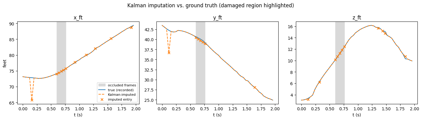
Optical tracking systems occasionally lose the ball for a few consecutive frames (occlusion by players, the rim, or a camera dropout), and can also miss scattered individual samples. We simulate both kinds of damage on a copy of the real arc:

• Occlusion: frames 15-19 (5 consecutive frames) are dropped entirely – every one of x_ft, y_ft, z_ft is NaN for those rows. This is exactly the gap that HyperTools’ default PPCA imputer cannot fill (GH #169): with zero observed features in a row, PPCA has nothing to condition its reconstruction on.

• Scattered noise: an additional ~10% of individual cells (seeded, for reproducibility) are set to NaN at random, simulating occasional single-camera dropouts.

We then run hyp.impute(damaged, model='Kalman') and compare the imputed values against the real, recorded ground truth.

rng = np.random.default_rng(42)

true_arc = arc.copy()
damaged = arc.copy()

OCCLUSION_SLICE = slice(15, 20)  # 5 consecutive fully-missing frames
damaged.iloc[OCCLUSION_SLICE, :] = np.nan

# ~10% scattered single-cell dropouts, only among the still-intact cells
intact_mask = ~damaged.isna().to_numpy()
scatter_frac = 0.10
n_scatter = int(round(scatter_frac * intact_mask.sum()))
intact_flat_idx = np.flatnonzero(intact_mask)
scatter_idx = rng.choice(intact_flat_idx, size=n_scatter, replace=False)
# NOTE: .to_numpy() can return a read-only, Fortran-ordered array; a plain
# .ravel() on that silently returns a *copy* (since it must reorder to C
# order), so writes through it would vanish. .copy() first (writable,
# C-contiguous) then index via .flat (always a real view) to guarantee the
# writes land.
damaged_values = damaged.to_numpy().copy()
damaged_values.flat[scatter_idx] = np.nan
damaged = pd.DataFrame(damaged_values, index=arc.index, columns=arc.columns)

n_missing = damaged.isna().to_numpy().sum()
print(f'damaged: {n_missing} / {damaged.size} cells missing '
      f'({100 * n_missing / damaged.size:.1f}%), including '
      f'{OCCLUSION_SLICE.stop - OCCLUSION_SLICE.start} fully-NaN rows '
      f'(frames {OCCLUSION_SLICE.start}-{OCCLUSION_SLICE.stop - 1})')
damaged.iloc[13:22]

damaged: 29 / 150 cells missing (19.3%), including 5 fully-NaN rows (frames 15-19)

	x_ft	y_ft	z_ft
t_s
0.519	73.52751	41.21501	9.05020
0.559	73.80681	40.93222	9.56722
0.599	NaN	NaN	NaN
0.640	NaN	NaN	NaN
0.679	NaN	NaN	NaN
0.719	NaN	NaN	NaN
0.760	NaN	NaN	NaN
0.799	76.15129	38.62498	12.99190
0.839	76.66918	38.04769	13.60741

import hypertools as hyp

imputed = hyp.impute(damaged, model='Kalman')

missing_mask = damaged.isna().to_numpy()
rmse_per_axis = np.sqrt(
    np.nanmean(
        np.where(missing_mask,
                 (imputed.to_numpy() - true_arc.to_numpy()) ** 2, np.nan),
        axis=0))
overall_rmse = np.sqrt(
    np.mean((imputed.to_numpy()[missing_mask] - true_arc.to_numpy()[missing_mask]) ** 2))

for col, r in zip(arc.columns, rmse_per_axis):
    print(f'  RMSE[{col}] = {r:.3f} ft (over {missing_mask[:, list(arc.columns).index(col)].sum()} imputed entries)')
print(f'Overall RMSE (all imputed entries, all axes): {overall_rmse:.3f} ft')

occlusion_rmse = np.sqrt(np.mean(
    (imputed.iloc[OCCLUSION_SLICE].to_numpy() - true_arc.iloc[OCCLUSION_SLICE].to_numpy()) ** 2))
print(f'RMSE restricted to the 5 fully-occluded frames: {occlusion_rmse:.3f} ft '
      '(this is the GH #169 gap PPCA cannot fill)')

  RMSE[x_ft] = 2.146 ft (over 11 imputed entries)
  RMSE[y_ft] = 2.124 ft (over 7 imputed entries)
  RMSE[z_ft] = 0.185 ft (over 11 imputed entries)
Overall RMSE (all imputed entries, all axes): 1.688 ft
RMSE restricted to the 5 fully-occluded frames: 0.202 ft (this is the GH #169 gap PPCA cannot fill)

Imputation, visualized

The dashed vertical band marks the fully-occluded frames (15-19); markers show every imputed entry (whether from the occlusion band or a scattered single-cell dropout) alongside the true recorded value.

fig, axes = plt.subplots(1, 3, figsize=(14, 4), sharex=True)

for ax, col in zip(axes, arc.columns):
    ax.axvspan(arc.index[OCCLUSION_SLICE.start], arc.index[OCCLUSION_SLICE.stop - 1],
               color='0.85', label='occluded frames' if col == 'x_ft' else None)
    ax.plot(true_arc.index, true_arc[col], color='C0', label='true (recorded)')
    ax.plot(imputed.index, imputed[col], color='C1', linestyle='--',
            label='Kalman-imputed')
    col_idx = list(arc.columns).index(col)
    miss_idx = np.flatnonzero(missing_mask[:, col_idx])
    ax.scatter(arc.index[miss_idx], imputed[col].to_numpy()[miss_idx],
               color='C1', marker='x', s=30, zorder=5, label='imputed entry')
    ax.set_title(col)
    ax.set_xlabel('t (s)')

axes[0].set_ylabel('feet')
axes[0].legend(loc='best', fontsize=8)
fig.suptitle('Kalman imputation vs. ground truth (damaged region highlighted)')
fig.tight_layout()

Part 2: Forecasting – extrapolating the arc’s remainder

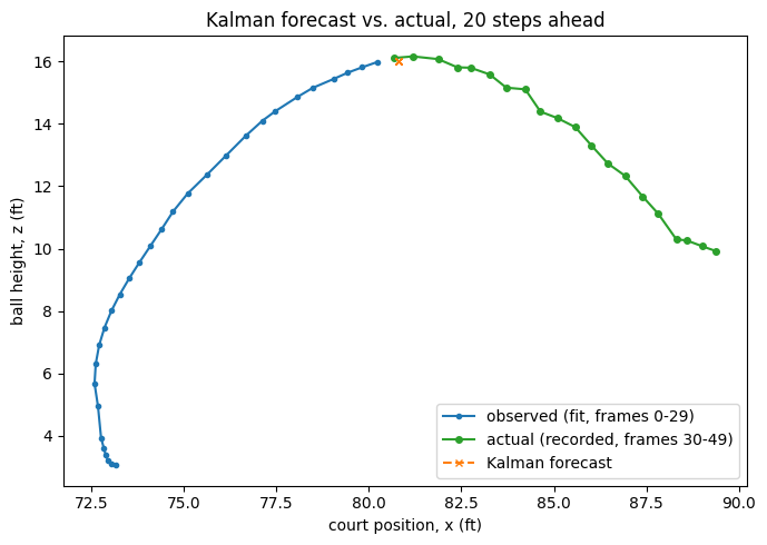
Now the other direction: given only the first 30 frames of the arc (the rising portion through just past the apex), can hyp.predict with a Kalman model extrapolate the remaining flight? We fit on frames 0-29 and forecast t=20 steps ahead, then compare against the actual, recorded final 20 frames.

FIT_FRAMES = 30
HORIZON = 20  # == len(arc) - FIT_FRAMES

first30 = arc.iloc[:FIT_FRAMES]
actual_tail = arc.iloc[FIT_FRAMES:FIT_FRAMES + HORIZON]

forecast = hyp.predict(first30, model='Kalman', t=HORIZON)

mae_per_axis = np.mean(np.abs(forecast.to_numpy() - actual_tail.to_numpy()), axis=0)
for col, m in zip(arc.columns, mae_per_axis):
    print(f'  MAE[{col}] = {m:.3f} ft')
print(f'Overall MAE (all axes): {np.mean(mae_per_axis):.3f} ft')

  MAE[x_ft] = 4.469 ft
  MAE[y_ft] = 5.579 ft
  MAE[z_ft] = 2.543 ft
Overall MAE (all axes): 4.197 ft

Forecast, visualized (side view: x vs. z)

Solid blue is the observed rising portion the model was fit on; solid green (with circle markers) is the actual recorded continuation; dashed orange (with x markers) is the Kalman forecast.

fig, ax = plt.subplots(figsize=(7, 5))
ax.plot(first30['x_ft'], first30['z_ft'], color='C0', marker='o',
        markersize=3, label='observed (fit, frames 0-29)')
ax.plot(actual_tail['x_ft'], actual_tail['z_ft'], color='C2', marker='o',
        markersize=4, label='actual (recorded, frames 30-49)')
ax.plot(forecast['x_ft'], forecast['z_ft'], color='C1', linestyle='--',
        marker='x', markersize=5, label='Kalman forecast')
ax.set_xlabel('court position, x (ft)')
ax.set_ylabel('ball height, z (ft)')
ax.set_title(f'Kalman forecast vs. actual, {HORIZON} steps ahead')
ax.legend(loc='best')
fig.tight_layout()

The same forecast in full 3D, via hyp.plot

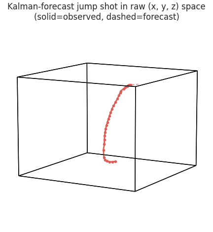
hyp.plot(..., predict='Kalman', t=...) overlays a dashed forecast tail directly on a HyperTools plot. Here we pass the raw (x, y, z) space through unreduced (reduce=None) since the data is already exactly 3 dimensions – the physical court-plane and height coordinates – so there’s nothing to project.

fig = hyp.plot([first30], predict='Kalman', t=HORIZON, reduce=None,
               fmt='-o', markersize=3, linewidth=2,
               title='Kalman-forecast jump shot in raw (x, y, z) space\n(solid=observed, dashed=forecast)')

Honest takeaways

A constant-velocity/acceleration Kalman model is a genuinely good fit for this problem because the underlying physics matches its assumptions: during free flight, gravity imposes constant acceleration, so position, velocity, and acceleration evolve linearly and the noise is well-described as Gaussian measurement jitter around a smooth trajectory. That’s exactly why it filled the fully-occluded frames well above (something the default PPCA imputer structurally cannot do, per GH #169) and extrapolated the ball’s continuing arc reasonably from only its rising half.

But the same assumptions that make it work here are exactly where it breaks down:

• Bounces and contact events (the ball hitting the rim, backboard, or floor) introduce near-instantaneous velocity discontinuities that a smooth linear-Gaussian model cannot represent – it will “round off” a bounce into a soft curve rather than a sharp reversal.

• Spin-induced effects (Magnus force from backspin, rim friction on contact) are nonlinear and not part of the constant-acceleration state space at all.

• Air drag technically makes free-flight deceleration horizontally velocity-dependent rather than perfectly constant, which the model approximates rather than models exactly (a minor effect at typical shot speeds, but not zero).

• Longer horizons amplify any of the above: small deviations from the ideal ballistic assumption compound the further the model is asked to forecast.

In short: trust a Kalman filter for the smooth, ballistic middle of a flight, and be skeptical of it across bounces, spins, or other contact events where the physics genuinely changes.

Next steps

• `hyp.impute API reference <../api.rst>`__ and the plot_impute gallery example.

• `hyp.predict API reference <../api.rst>`__ and the plot_predict gallery example.

• The stock forecasting tutorial applies the same hyp.predict API to a much less physically-constrained (and much harder) forecasting problem: daily equity prices.