Analyze¶

Import packages¶

import hypertools as hyp
import seaborn as sb
import matplotlib.pyplot as plt

%matplotlib inline

Load your data¶

First, we’ll load one of the sample datasets. This dataset is a list of 2 numpy arrays, each containing average brain activity (fMRI) from 18 subjects listening to the same story, fit using Hierarchical Topographic Factor Analysis (HTFA) with 100 nodes. The rows are timepoints and the columns are fMRI components.

See the full dataset or the HTFA article for more info on the data and HTFA, respectively.

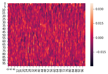
geo = hyp.load('weights_avg')
weights = geo.get_data()
print(weights[0].shape) # 300 TRs and 100 components
print(weights[1].shape)

(100, 100)
(100, 100)

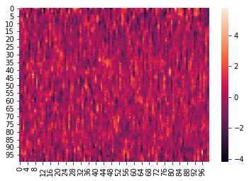
We can see that the elements of weights each have the dimensions (300,100). We can further visualize the elements using a heatmap.

for x in weights:
    sb.heatmap(x)
    plt.show()

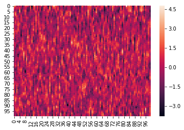
Normalization¶

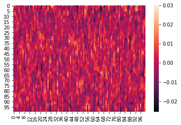
Here is an example where we z-score the columns within each list:

Normalize accepts the following arguments, as strings: + ‘across’ - z-scores columns across all lists (default) + ‘within’ - z-scores columns within each list + ‘row’ - z-scores each row of data

norm_within = hyp.analyze(weights, normalize='within')

We can again visualize the data (this time, normalized) using heatmaps.

for x in norm_within:
    sb.heatmap(x)
    plt.show()

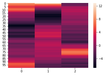
Normalize and reduce¶

To easily normalize and reduce the dimensionality of the data, pass the normalize, reduce, and ndims arguments to the analyze function. The normalize argument, outlined above, specifies how the data should be normalized. The reduce argumemnt, specifies the desired method of reduction. The ndims argument (int) specifies the number of dimensions to reduce to.

Supported dimensionality reduction models include: PCA, IncrementalPCA, SparsePCA, MiniBatchSparsePCA, KernelPCA, FastICA, FactorAnalysis, TruncatedSVD, DictionaryLearning, MiniBatchDictionaryLearning, TSNE, Isomap, SpectralEmbedding, LocallyLinearEmbedding, and MDS.

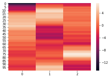
norm_reduced = hyp.analyze(weights, normalize='within', reduce='PCA', ndims=3)

We can again visualize the data using heatmaps.

for x in norm_reduced:
    sb.heatmap(x)
    plt.show()

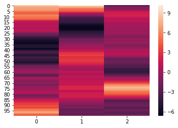
Finer control¶

For finer control of the model parameters, reduce can be a dictionary with the keys model and params. See scikit-learn specific model docs for details on parameters supported for each model.

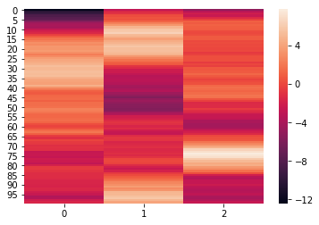
reduce={'model' : 'PCA', 'params' : {'whiten' : True}} # dictionary of parameters
reduced_params = hyp.analyze(weights, normalize='within', reduce=reduce, ndims=3)

We can again visualize the data using heatmaps.

for x in reduced_params:
    sb.heatmap(x)
    plt.show()

Normalize, reduce, and align¶

Finally, we can normalize, reduce and then align all in one step.

The align argument can accept the following strings: + ‘hyper’ - implements hyperalignment algorithm + ‘SRM’ - implements shared response model via Brainiak

norm_red_algn = hyp.analyze(weights, normalize='within', reduce='PCA', ndims=3, align='SRM')

Again, we can visualize the normed, reduced, and aligned data using a heatmap.

for x in norm_red_algn:
    sb.heatmap(x)
    plt.show()